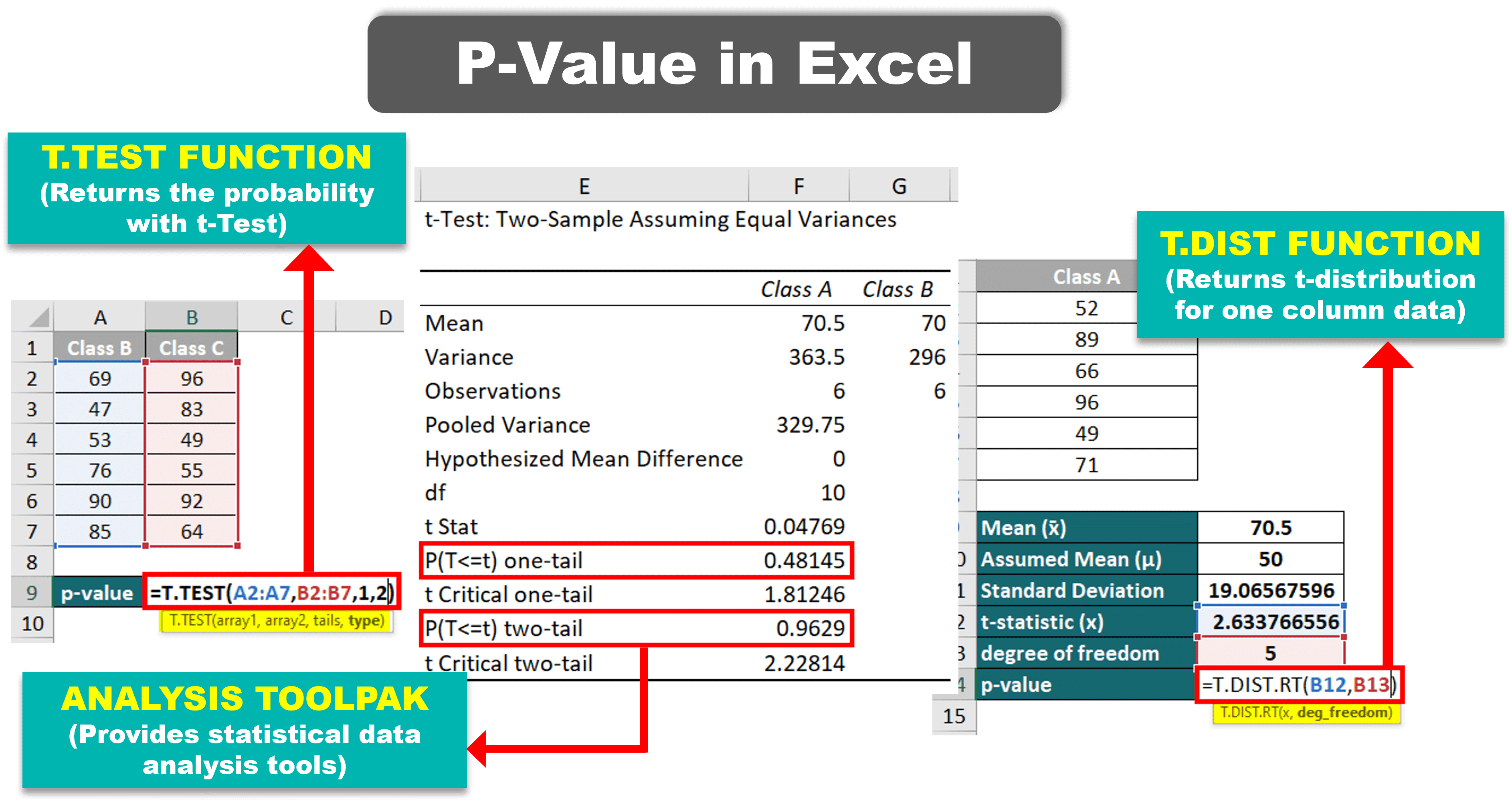
You don’t need a lab coat or a stats degree. Excel has a function literally called T.TEST. It sounds intimidating, but it’s just a machine that spits out your P-value. You feed it two sets of numbers—like “Sales Before vs. After Your Coffee” or “Test Scores with vs. Without Naps”—and it does the math.
The syntax is deceptively casual: =T.TEST(array1, array2, tails, type). “Tails” just means whether you’re checking for a difference in one direction (like “only higher?”) or both directions (“higher or lower?”). Most of the time, you’ll use 2 tails, because life is rarely one-sided.
And the “type” part? That’s where you tell Excel if your data is like twins (paired), cousins (equal variance), or strangers (unequal variance). Most of us just use 2 for equal variance because it’s the middle ground. Like ordering “medium” coffee—works for most situations.
 A Comprehensive Guide to Calculating P-Values in Excel - Earn and Excel
The “Ah-Ha” Moment
I remember the first time I actually used it. I was comparing website traffic on Tuesdays vs. Thursdays. I thought Tuesday was obviously better. I plugged in the ranges, pressed Enter, and got a P-value of 0.67.
That number basically screamed at me: “Dude, that difference is pure noise! Go drink your water and stop overthinking.” It saved me from creating a whole presentation based on a fluke. Now I joke that P-values are the protocol droid of data—they keep your ego in check.